The Average Crap*

I Collect puzzles and am the holder in due course of the family collection. My father stored this collection in a box made by my great grandfather.

I out grew the box years ago.

At one point I had a tangram puzzle. I’ve misplaced it so I made one.

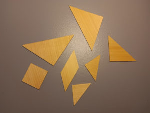
As you can see trangrams are a collection of seven specific
shapes. There are:

– Two large triangles
– One medium triangle
– Two small triangles
– A Parallelogram

Their purpose is to arrange them in pleasing patterns.

For instance, here is a dragon

My purpose is not to show how they might be arranged, but rather how to make a set. Other on-line instructions I’ve read thinks about paper or card stock. I chose wood.

I went to a craft store for a craft board. I found an eight inch square of basswood, 1/8th of an inch thick, perfect for my purposes. The basswood is soft enough to cut with patience and a mat knife and strong enough to stand up to this use.

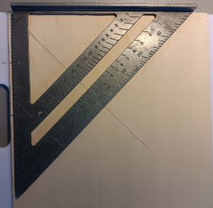
I found my cutting board in the kitchen (don’t tell Kate) and rooted around in my tool box for a triangle.

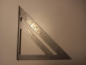
There is a six inch rule along the bottom leg and a flange on the other leg. Hold the flange along the edge of the cutting board to get either a right angle or a 45 degree angle.

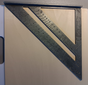
Now we’re ready to layout our cuts.

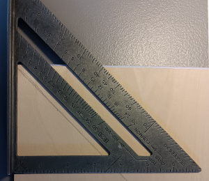
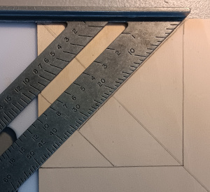
1. Place the flange along the top of the board with the 45 degree leg going through the top left corner of the board. Draw that diagonal.

2. Measure along the side edge to the desired width. Mark that point The largest triangle will have this distance as the hypotenuse of their legs. I chose four inches.

3. Mark the half way point. I calculated two inches.

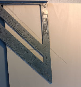
4. Move the triangle so the the pivot point is at the desired width and the right angle leg goes across the board. Draw a line to the diagonal drawn in step one.

5. With the triangle flange along the top of the board, move triangle so that the right angle leg meets the intersection of the diagonal and bottom edge drawn in step four. You’ve now laid out a square which we will cut into tans (each piece of a tangram is called a
tan).

6. With the triangle flange along the side of the board move the the other point to the half-way mark. Draw a diagonal parallel to the first (and half its length) to the bottom of the
square. Confirm that it in fact crosses the bottom at the half-way point.

7. Get out your mat knife and cut out the square. I found that I had to score the wood using the right angle leg of the triangle to steady my blade. I kept running my knife through those scores until it broke through.

8. Draw a diagonal, perpendicular to the first through the top right corner. The line should go no than further the second, shorter, diagonal. You have now laid out the two large triangles and the one mid-sized triangle at the opposite corner. We will lay out
the other pieces in the band between the large triangles and the mid-sized.

9. Place the triangle flange along the top of the board so that the right angle leg goes through the intersection of the second and third diagonals. Draw a line from the third diagonal to that point laying out the parallelogram and one small triangle.

10. Slide the triangle (with the flange along the side) so that hypotenuse leg meets the intersection of the second diagonal and the base. Draw a line from that point to the third diagonal laying out the square and the second small triangle.

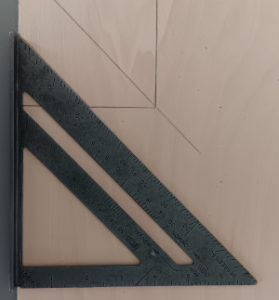
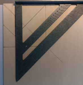
Your layout should look like this:

Cut, in the following order:
– The first diagonal.
– The second (shortest) diagonal
– The third diagonal bisecting the largest piece into two large triangle.
– The third diagonal through that band yielding two quadrilaterals.
– The line between the parallelogram and a small triangle
– The line between the square and a small triangle

There are fourteen solid shapes that can be assembled using all the tans. A shape is solid if there are no lines between two points on its perimeter that cross an empty space.

I’ve read there are 9500 designs one can make using all seven pieces.  All must lay flat.

I just turned off comments and I’m sorry.

I get an email for each comment submitted.  I’ve approved one.  All of the others were spam and I got tired of logging in and moving them to trash.

In 1976, with my brand-new bachelors degree hanging on the wall of my bedroom [I wanted to put it in the bathroom—KD], I started work at a Big Eight CPA firm. I had spent the previous four years preparing customs tax returns and had lots of experience with desktop calculators. Nonetheless, I was unprepared for the twenty-page computer report whose total I had to prove.

I borrowed an adding machine from the client and set to work. A day later I had an impossibly long tape showing the same total as the report. I marked it with an f (for footed [accountant-speak for checked and proved—KD]) on the report and went to the next task.

I discovered that I was constitutionally incapable of correctly adding more than twenty numbers on the first try. It was my policy to run two tapes and compare them. I needed a better way.

I wrote Hot Footer in 2014 and have been using it ever since. Hot Footer is that same calculator as in 1976 without the mechanical clack but with a tape I can copy and paste.

This last month it occurred to me that I ought to share Hot Footer; hence the website with a download link. Hot Footer is written in Java, and therefore you must have installed the Java run-time engine (JRE). You can find it at https://www.oracle.com/java/technologies/downloads/. Click on JRE for Consumers.

For those whose experience is with algebraic calculators, Hot Footer will take some time to get used to, but if you routinely add long columns, it will be worth the effort.

Multiplication and division work as with any algebraic device. Enter a number, an operator, and another number, and hit equals. Hot Footer puts all that on the tape and produces a total:

For addition and subtraction, enter the number followed by its sign. Hot Footer places that entry on the tape, black for positive and red for negative. Once the final entry has been made, equals (or the enter key) causes Hot Footer to print the total.

My fingers know this routine. Someone long ago introduced me to the little bump on the five, a locator bump just like the bumps on the F and J keys. Don’t look; feel for the button on the ten-key pad to orient your fingers on the 4, 5, and 6. I’m so used to the rhythm—number, operator, number, operator—that hear the adding machine clack just as it did in the 70s. .

This is a posting on evaluating financial statements. Beneish M Score is a calculation to determine how likely it is that a statement is fraudulent. Generally the score is negative. As long as its is less than –1.78, the probability of fraud is low.

The score was developed by Messod Daniel Beneish, professor of accounting at the Kelley School of Busines at Indiana University.

The calculation for 3M for the year ended February 8, 2023, is

My conclusion, based on the score of –2.40, is that these statements are unlikely to contain fraud.

The score is the weighted total of eight indices.

The first index is day’s sales in receivables, a ratio of accounts receivable to sales divided by 365; it is a usual financial statement ratio. It shows on average how long it takes the company to collect its revenues. The index is the ratio of the current year to the prior one. If the company is recording sales that don’t exist, this should be greater than one.

The second index is gross margin index, that is, sales less cost of sales. Many financial statements show this as a subtotal on the income statement. The index is this year’s gross margin as a percent of sales to last year’s. Beneish believes that a declining margin is motivation for creative accounting.

The third is asset quality index. In some sense every asset is held to produce income. Each asset but cash and receivables has a life and should get written off over that life. Beneish identifies assets whose life and contribution to operations is clear. Those are current assets; plant, property, and equipment (PP&E); and securities, or quality assets. The asset quality ratio is (total_assets – quality_assets) ÷ total_assets.

Fourth is the sales growth index. That is this year’s sales to last year’s. Beneish believes that increasing sales may motivate management to overstate income in years when income does not meet expectations.

Fifth is depreciation index, the ratio of the percentage of PP&E written off this year to last. Overstating the value of PP&E and understating the depreciation charge are both techniques of managing income that are not generally accepted.

Selling, general, and administrative costs (SG&A) are the source of the next index. This year’s SG&A as a percent of sales is divided by last year’s. Subtract this index.

The leverage index, item 7, is the ratio of current liabilities plus long-term debt to total assets. It is a current-year statistic only. Beneish believes that highly leveraged firms are particularly likely to overstate income. Subtract this index from the score.

The last index is accruals to assets. That is (Cash provided by operations – Operating income)/Total Assets. Beneish’s observation is that misstatements rarely affect cash and therefore contribute to the difference between income and cash flow.

I wrote a workspace to perform this calculation. You can find it here. Fill in the array Beneish input. The function bi_Beneish_M will return the score and bi_Beneish_M_report will show the calculation of the score.

I found many websites explaining the Beneish M score and how to calculate it. Many noted that Enron scored in the fraud likely range but no one paid attention. Few websites actually offered a set of financial statements and calculated the M score.

One website that did calculate the M score got it wrong. The assets quality index (which measures the assets without quality [unquality being not a word.—KD]) was calculated with the quality assets as the numerator of the ratio. Their data was also flawed, as quality assets were greater than total assets.

~This all leads to my tentative conclusion: the Beneish M score, while it has demonstrated the ability to predict fraud, is too complicated. Beneish himself acknowledged that his eponymous score has too many false positives that require a great deal of digging to resolve.

My old laptop computer died, so I went and bought a new one. It arrived almost in time for my birthday, so the time I’ve spent setting it up was my birthday present.

Or rather I tried to convince myself that I was enjoying the challenge.

I have many happy memories of new computers with new or updated operating systems and discovering the innovative features of my new machine.

The last time I found that was with a Windows 3.1 computer. I had gotten my feet wet with a graphical interface, as one of my clients used Macs.

I was more than ready for running multiple programs at the same time and jumping from one to another. At that time I had a client who still posted his books by hand. Each time I went to see him, he presented me with a trial balance handwritten on ledger paper, and I dutifully copied everything into a file on my hard drive.

He in fact needed Windows more than I did. He had two desks, both covered with papers and open ledgers. He, like me, needed to refer to many sources as his work progressed; hence the second desk.

Unpacking my new box, I expected a voyage of discovery as I got the thing running, completely ignoring every version of Windows since version 3.1. Microsoft confuses change with innovation and thus changes the interface with each new version with little or no actual additional (or improved; often the opposite—KD) function. My voyage crashed on the rocks as the Windows logo opened on the laptop.

I had planned to make this a dual-boot machine, Linux or Windows. Step one was make a Windows recovery disk, and step two was install some basic applications, with Emacs and Open Office at the top of the list. I struggled and finally got to installing Linux.

Linux refused to partition the hard drive, which apparently Windows encrypts.. I got to a website that would “explain”—they fondly suppose—how to deal with the encryption. I gave up. I’m not a Windows fan anyway.

I still hadn’t given up hope of encountering some innovative features. I dove into the Linux install process. It didn’t take long to have a functioning laptop again. It was something of a relief that I had an administrator login and a user login, something still absent from Windows.

I started using Linux in the early 90s and have not looked back. Many years have brought a better install process, so the tedious things like partitioning and formatting the disk are done for you. Every year brings some new application or feature, and I’ve adopted many of them. All require installation and configuration. So while I quickly got back a working computer, I’ve spent the past two days installing the applications I wanted.

In terms of discovery, I discovered that Window Maker is spelled wmaker (Ugh—KD). We won’t discuss how long that discovery took or how many dead ends I went up in the discovery process.

I guess in some perverse way I still miss Windows 3.1. (It’s hardly perverse if it’s logical and reasonable.—KD)

Continue reading →

This post is a follow up to *Crunching Numbers in APL* available for kindle at Amazon.

Undaunted by my last foray into online analytical processing (OLAP), I sat down to code what I thought was OLAP. Workspace more_olap is here.

Should you load this workspace, you will find the following variables:

A fact in this exercise is the line item and amount columns from irdb.

irdb is made up of these columns:

      utl∆numberedArray ⊃ irdb[1;]
[001] Category code
[002] Category
[003] Subcategory code
[004] Subcategory
[005] Line item
[006] Fiscal year
[007] Amount (millions of dollars)

The function olap∆buildFacts loads the irdb data and produces all of these variables. You should also consider olap∆buildVars, which will produce variables to use as indices of facts.

      olap∆buildVars cats subs yrs
      )vars cat_
cat_a   cat_e   cat_l
      )vars sub_
sub_b       sub_cs  sub_da  sub_dfb     sub_dl      sub_i       sub_lo  sub_nn
sub_o       sub_oa  sub_oe  sub_ol      sub_orcv    sub_rcv     sub_re  sub_s
sub_sol
      )vars yr_
yr_2009     yr_2010

We now have some variables to use as indices of our fact cube and can look at our cube:

      olap∆combineFacts facts[cat_e;yr_2010]
 Paid-in capital                      11492
 Retained earnings                    28793
 Accumulated other comprehensive loss ¯3043

      ⍝ Or
      +/(olap∆combineFacts facts[cat_e;yr_2010])[;2]
37242

I still haven’t concluded that it’s easier than this:

SELECT Line_item, Amount from irdb where Category_code = 'e'
and Fiscal_year = 2010;

But I’m biased. While I’ve been writing APL code longer, I’ve spent more time writing SQL.

This is a simple exercise with simple data. It demonstrates what a data cube might look like and how to simplify slicing and dicing the data. There is no generalized code in this workspace, and therefore I must write a whole new workspace when I want to analyze a new data set.

I’m reminded of the weeks I spent designing a gross margin reporting system for a manufacturer. This company had several product lines and three departments. It had detailed time reports from the factory floor, so that I knew how much labor cost was incurred by product line and by department. It had a perpetual inventory system, so that I knew what material had been drawn from raw material inventory and production counts for each department. This allowed me to construct a model of the manufacturing process and estimates of costs incurred through each step in that process.

I’d like to get my hands on that long-lost data and see if a data cube would simplify anything.

OLAP stands for OnLine Analytical Processing. This post describes why
I’m not ready to write about OLAP.

I’ve been reading various web pages about OLAP and have reached two
conclusions. First, the demand for OLAP is driven by SQL commands’
complexity, which can arise when the programmer is querying complex
databases. Nontechnical users stumble badly in that environment, and
even correct queries can take too long to execute.

Second, the processing is done on a new non-SQL database designed to
make querying easier and processing time faster. Generally, this means
an underlying SQL database is kept to record transactions, and an OLAP
database is updated periodically from the SQL database. The OLAP
database usually is an array of facts determined by the SQL queries.
Each dimension of the array is a fact attribute for which aggregate data
may be sought.

I’ve been struggling to a third conclusion, that I can reach a better
understanding of the data by investigating why and how the data was
compiled than by constructing complicated SQL queries.

I found an open-source OLAP application, Cubes, written in
python([[http://cubes.databrewery.org/]]). I downloaded the application
and started on the tutorial. Step one, called Hello World, constructs a
data cube from balance sheets of the International Bank for
Reconstruction and Development for the years 2010 and 2011.

I was planning to code an OLAP database in APL, so rather than following
the tutorial, I just loaded the supplied csv file into APL.

      ibrd←import∆file 'Downloads/IBRD_Balance_Sheet__FY2010.csv'
      ⍴ibrd
63 7

That didn’t look like a lot of data, so I displayed some of it:

      ibrd[⍳5;]
 Category Code Category Subcategory Code Subcategory    Line Item                         Fiscal Year Amount (US$, Millions) 
 a             Assets   dfb              Due from Banks Unrestricted currencies                  2010                   1581 
 a             Assets   dfb              Due from Banks Unrestricted currencies                  2009                   2380 
 a             Assets   dfb              Due from Banks Currencies subject to restriction        2010                    222 
 a             Assets   dfb              Due from Banks Currencies subject to restriction        2009                    664 

My seven columns:

1. Category code
2. Category
3. Subcategory code
4. Subcategory
5. Description (called line item above)
6. Fiscal year
7. Amount (in $US millions)

I concluded that our cube should have two dimensions, description and
year. Each fact (cell in the array) should be made up of a description
and an amount. The category Descriptions is a hierarchy of category,
subcategory and item.

With that in mind I dived off the cliff and started writing APL queries.
Question one always is whether the debits equal the credits, or in this
case whether total assets equal total liabilities plus total equities.

I needed to confirm that both years and amounts were in fact numbers:

      utl∆numberp ¨ 1 0↓ibrd[⍳10;6 7]
1 1
1 1
1 1
1 1
1 1
1 1
1 1
1 1
1 1

Yes.
I knew I’d get tired of the column heads, so I copied the array without
them.

      db←1 0 ↓ibrd

I also determined the universe of category codes to simplify my next
query.

      db[;1]
 a a a a a a a a a a a a a a a a a a a a a a a a a a a a a a a a l l l l l l l l l l l l l l l l l l l l l l e e e e e e e e 

I concluded that *a* means assets, *l* means liabilities, and *e* means
equity. My queries:

      +/(∊db[;1]='a')/db[;7]
558430
      +/(∊db[;1]='l')/db[;7]
480838
      +/(∊db[;1]='e')/db[;7]
77592
      480838 + 77592
558430

I started planning my next query and was curious: what descriptions
describe each fact?

      ⍞←⎕tc[3] utl∆join (db[;6]=2010)/db[;5]
Unrestricted currencies
Currencies subject to restriction
Trading
Securities purchased under resale agreements
Nonnegotiable, nonintrest-bearing demand obligations on account of subscribed capital
Investments
Client operations
Borrowings
Other
Receivables to maintain value of currency holdings on account of subscribed capital
Receivables from investment securities traded
Accrued income on loans
Net loans outstanding
Assets under retirement benefit plans
Premises and equipment (net)
Miscellaneous
All
Securities Sold under Repurchase Agreements, Securities Lent under Securities Lending Agreements, and Payable for Cash Collateral Received
Investments
Client Operations
Borrowings
Other
Payable to Maintain Value of Currency Holdings on Account of Subscribed Capital
Payable for investment securities purchased
Accrued charges on borrowings
Liabilities under retirement benefit plans
Accounts payable and misc liabilities
Paid-in capital
Deferred Amounts to Maintain Value of Currency Holdings
Retained Earnings
Accumulated Other Comprehensive Loss

I stopped.

I am not a bank accountant, so I must open the accounting rulebook and
read it cover to cover before I try to read banks’ financial statements.

Let’s consider a few facts. Accumulated other comprehensive loss is an
equity account that accumulates unrealized gains and losses. What they
might be is in the financial statements. We have just one page.

The subcategories make matters worse.

       ⍞←⎕tc[3] utl∆join (db[;6]=2010)/db[;4]
Due from Banks
Due from Banks
Investments
Securities
Nonnegotiable
Derivative Assets
Derivative Assets
Derivative Assets
Derivative Assets
Receivables
Other Receivables
Other Receivables
Loans Outstanding
Other Assets
Other Assets
Other Assets
Borrowings
Sold or Lent
Derivative Liabilities
Derivative Liabilities
Derivative Liabilities
Derivative Liabilities
Other
Other Liabilities
Other Liabilities
Other Liabilities
Other Liabilities
Capital Stock
Deferred Amounts
Retained Earnings
Other

When the Financial Accounting Standards Board issued guidance on
derivatives, I passed. I could do better in Atlantic City than with
derivatives, and so how to account for them was irrelevant. It certainly
seemed probable that these liabilities give rise to some of the
accumulated other comprehensive losses.

So after I complete my study of the accounting rules, I need to digest
the footnotes to the financial statements to get some understanding of
four different kinds of derivatives.

I have yet to extract an analysis of the facts I have. And that’s why
I’m not writing about OLAP…yet.
Continue reading →

When I took Accounting 1, I dreamed ledgers. In those days most medium to small companies kept their books by hand and stored them in a fireproof safe. One of the requirements of the course was a complete set of books consisting of financial reports for a fiscal period. It was all done by hand on ledger paper. I did manage to do some of it at work, where I could use a claculator [sic].

The dreams helped internalize accounting, and to this day if I have a difficult accounting problem, I’ll start with ledger paper and lay out my solution. At some point I’ll see the solution and then complete my work in APL.

What this means is that I am not afraid of long columns of figures nor of large arrays. I can extract insights just by examining the reports and doing some simple arithmetic.

Most people need something more, and a well-designed graph is always helpful. Accordingly, this post describes how to produce a graph in GNU APL and how to dress it up for company.

Graphing is not part of the ISO standard, but many APL interpreters provide a graphing function. In GNU APL it is ⎕plot. The syntax is attributes ⎕plot data. The handle return by ⎕plot is an integer that identifies the graph. Close the window with ⎕plot handle.

The data is what will be plotted. For a vector of real numbers, the data point will be positioned along the Y axis, and its position along the X axis by its position in the vector. Plotting according to pairs of data is done using complex numbers, which are the sum of a real number and an imaginary number. Thus, for a two-column array we could produce a graph by converting each row to a complex number:

      ⎕plot a_b[;1] + 0j1 × a_b[;2]

Dressing graphs up for company requires setting attributes. ⎕plot ” will give you a list of attributes.

I got into a heated discussion recently about U.S. tax policy, which led to the graph we’re about to construct.

I downloaded my data from BEA.gov and imported it into APL:

      income_expense_raw←import∆file '/home/dalyw/AverageCrap/Research/Federal_I_E.csv'
      gdp_raw←import∆file '/home/dalyw/AverageCrap/Research/GDP_2017Q1_2022Q4.csv'

For our purposes all we want is gross domestic product, line 6 in gdp_raw, and federal receipts, line 6 in income_expense_raw.

      gdp←gdp_raw[6;2↓⍳25]
      fed_receipts←income_expense_raw[6;2↓⍳25]

We want to plot both statistics against an actual timeline so that the X axis labels show quarterly increments.

      SPQ←×/91 24 60 60		⍝ Seconds in one quarter
      q1←⎕fio.secs_epoch 2017 2 15
      time←q1 + SPQ × ¯1 + ⍳23

We build the attribute array:

      ⍝ Set the GDP line color to blue
      att_gdp_tax.line_color_1←'#0000FF'
      ⍝ Set the tax line to green
      att_gdp_tax.line_color_2←'#00FF00'
      ⍝ Set the legend to identify both lines
      att_gdp_tax.legend_name_1←'Gross Domestic Product'
      att_gdp_tax.legend_name_2←'Tax receipts'
      ⍝ Position the legend away from the two lines
      att_gdp_tax.legend_X←50
      att_gdp_tax.legend_Y←200
      ⍝ Set the caption to identify the graph
      att_gdp_tax.caption←'US GDP and Tax Receipts in Billions'
      ⍝ Set the format of the X-axis labels to show year and quarter
      att_gdp_tax.format_X←'%yQ%Q'

Now we can call ⎕plot:

      att_gdp_tax ⎕plot (time + 0j1 × gdp),[0.1] time + 0j1 × fed_receipts

Quod erat demonstrandum.

This is post three of my Crunching Numbers in APL series. I’m
returning to my database of the top twenty stocks in the
Standard and Poor’s 500.

      sp20[;1 2 3 4 7]
 Symbol Name                        Price    Div $    FCF 
 WMT    Walmart                    142.09     2.28 ¯10929 
 AMZN   Amazon                      95.82     0     ¯1112 
 AAPL   Apple                      149.4      0.92  ¯2343 
 CVS    CVS Health                  86.04     2.42   2832 
 UNH    UnitedHealth Group         488.17     6.6    8651 
 XOM    Exxon Mobil                110.74     3.64  28024 
 BRK-B  Berkshire Hathaway         300.69     0         0 
 GOOG   Alphabet                    91.07     0         0 
 MCK    McKesson                   360.33     2.16      0
 ABC    AmerisourceBergen          159.5      1.94      0 
 COST   Costco Wholesale           493.14     3.6       0 
 CI     Cigna                      295.65     4.92      0 
 T      AT&T                        19.25     1.11      0 
 MSFT   Microsoft                  254.77     2.72      0 
 CAH    Cardinal Health             77.7      1.98      0 
 CVX    Chevron                    161.93     6.04      0 
 HD     Home Depot                 299.31     8.36      0 
 WBA    Walgreens Boots Alliance    36.21     1.92      0 
 MPC    Marathon Petroleum         125.52     3         0 
 ELV    Elevance Health            486.12     5.92      0 
 KR     Kroger                      43.91     1.04      0 
 F      Ford Motor                  12.07     0.6       0 
VZ     Verizon Communications      38.53     2.61      0

You’ll note I’ve added a column with some data. FCF is Free Cash
Flow. I’m using my own definition. I hope that it will act as
sieve to highlight stocks which deserve a closer look.

First I’d like to discuss databases. Chapter 11 of Crunching
Numbers in APL applies the principles of database design to APL
variables. We’re not to that point. We’re still in discovery
mode.

I set up a workspace for my research into companies that do not
pay dividends it includes the table sp20 shown above. As I’ve
done calculations I’ve tried to save those calculations and the
workspace as I played with Free Cash Flow. Here is where I
stand:

      )vars
aapl_free_cash      amzn_free_cash  cvs_free_cash   date∆US
date∆cal            date∆dates      date∆delim      date∆time∆M
date∆time∆delim     date∆time∆utce  date∆tz         final_vym
free_cash           g_data          g_return        goog
goog_covar          goog_free_cash  goog_hist       goog_variance
s_data              s_return        sp20            sp500
sp500_df            tmp             unh_free_cash   v_divs
v_lillian           vd_lillian      voo             vym
vym2                vym_div         vym_hist        wmt_free_cash
xom_free_cash

All the variables that begin date∆ belong the to
the date workspace in library 3 DALY and I’ll ignore them.

The variables sp500..., goog...,
and vym... were used for last week’s post on zero
dividend. The variables that end free_cash are for
today’s column.

APL’s workspace concept allows us this luxury. As I explore a
subject I can save my work in variables. They just exist and
don’t get in the way once I move on to something else.

For this project I created the variable free_cash and the
function calc_free_cash.

      free_cash
 Cash from operations       0 
 Interest                   0 
                      ------- 
 Adj Cash from ops          0 
 Capital exp                0 
 Dividends paid             0 
 Debt serv                  0 
 Stock repurchases          0 
                       ------ 
 Free cash                  0 
                      ======= 
 Debt service                 
 Interest                   0 
 Debt repayment             0 
 other                      0 
                      ------- 
                            0 

     ∇rs←calc_free_cash fc                                              
[001] ⍝ Function calculate free cash flow from a free_cash 
[002] ⍝ workpaper and returns a free_cash workpaper with 
[003] ⍝ those results.               
[004] rs←fc                                                             
[005] rs[4;2]←+/rs[1 2;2]                                               
[006] rs[13;2]←-rs[2;2]                                                 
[007] rs[7;2]←rs[17;2]←+/rs[13 14 15;2]                                 
[008] rs[10;2]←+/rs[4 5 6 7 8;2]                                        

My idea is a measure of the cash available from the operations
that can be used to grow the company. Today’s Wall Street
Journal has an article on evaluating companies that pay
dividends. It recommends ignoring the amount of the dividend and
instead focusing on cash flow.

The financial statements have five basic statements:

• Balance Sheet
• Income Statement
• Comprehensive Income
• Stockholder’s Equity
• Cash flow

My free cash flow calculation pulls amounts from that last
statement, Cash flow. Its worth looking the statement as whole.

First it reconciles net income to cash from operations. That
reconciliation includes items used to calculate net income which
do not use or provide cash, depreciation for example. The
reconciliation also includes changes in working capital that
require or provide cash.

Second it shows investment activity. I get my capital
expenditures from this section. I know that the company must
replace plant, property and equipment as it wears out. I use
this line as an estimate for future operations.

Third it shows financing activity, debt and equity
transactions. Here I find the amount of dividends paid and stock
repurchased. I calculate debt service as interest (from the
income statement) plus debt repayment for this section of the
cash flow statement.

The decision to finance the company through debt requires
consideration of the payment of interest and the retirement of
principle. I recognize this by adding interest to cash from
operations, and including it in debt service.

Many things may be said about this approach. It is
too simple. A thorough reading the financial statements and
Management’s Discussion and Analysis of Financial Condition and
Results of Operations might yield better estimates. In fact
those estimates my be buried in the 10-K somewhere.

This method is quick and dirty but I like it.

MCK, McKesson, is next on my list. I found its 10-K for the year
ended March 31, 2022 at www.sec.gov and its statement of cash
flow on page 74. Here is how I calculate free cash flow.

      mck_free_cash←free_cash
      mck_free_cash[1;2]←4434
      ⍝ This from the bottom of the cash flow statement
      mck_free_cash[2;2]←186	
      ⍝ The total of property, plant and equipment and software
      mck_free_cash[5;2]←¯388 + ¯147 
      mck_free_cash[6;2]←¯277
      ⍝ Repayment of long-term debt and debt extinguishments
      mck_free_cash[12;2]←¯1648 + ¯184 
      mck_free_cash[8;2]←¯3516

      ⍞←mck_free_cash←calc_free_cash mck_free_cash
 Cash from operations    4434 
 Interest                 186 
                      ------- 
 Adj Cash from ops       4620 
 Capital exp             ¯535 
 Dividends paid          ¯277 
 Debt serv              ¯2018 
 Stock repurchases      ¯3516 
                       ------ 
 Free cash              ¯1726 
                      ======= 
 Debt service           ¯1832 
 Interest                ¯186 
 Debt repayment             0 
 other                      0 
                      ------- 
                        ¯2018 

Now I’ll update my database and cross McKesson of my list.

      sp20[10;]
 MCK McKesson 360.33 2.16 21.79 263966 0 
      sp20[10;7]←¯1726
      sp20[;1 2 3 4 7]
 Symbol Name                        Price    Div $    FCF 
 WMT    Walmart                    142.09     2.28 ¯10929 
 AMZN   Amazon                      95.82     0     ¯1112 
 AAPL   Apple                      149.4      0.92  ¯2343 
 CVS    CVS Health                  86.04     2.42   2832 
 UNH    UnitedHealth Group         488.17     6.6    8651 
 XOM    Exxon Mobil                110.74     3.64  28024 
 BRK-B  Berkshire Hathaway         300.69     0         0 
 GOOG   Alphabet                    91.07     0         0 
 MCK    McKesson                   360.33     2.16  ¯1726 
 ABC    AmerisourceBergen          159.5      1.94      0 
 COST   Costco Wholesale           493.14     3.6       0 
 CI     Cigna                      295.65     4.92      0 
 T      AT&T                        19.25     1.11      0 
 MSFT   Microsoft                  254.77     2.72      0 
 CAH    Cardinal Health             77.7      1.98      0 
 CVX    Chevron                    161.93     6.04      0 
 HD     Home Depot                 299.31     8.36      0 
 WBA    Walgreens Boots Alliance    36.21     1.92      0 
 MPC    Marathon Petroleum         125.52     3         0 
 ELV    Elevance Health            486.12     5.92      0 
 KR     Kroger                      43.91     1.04      0 
 F      Ford Motor                  12.07     0.6       0 
 VZ     Verizon Communications      38.53     2.61      0 
 JPM    JPMorgan Chase             139.67     4         0 
 GM     General Motors              39.25     0.36      0